Lecture 3

• Welcome!
• Defining Functions
• Scope
• Checking Input
• Loops
• Using Loops
• Using Functions and Loops
• Applying Functions
• Summing Up

Welcome!

• Welcome back to CS50’s Introduction to Programming with R!
• Today, we will be learning about applying functions. We will also learn how to write our own functions and apply loops.

• Recall a program that we created during our last lecture called count.R.

  # Demonstrates counting votes for 3 different candidates
  
  mario <- as.integer(readline("Mario: "))
  peach <- as.integer(readline("Peach: "))
  bowser <- as.integer(readline("Bowser: "))
  
  total <- sum(mario, peach, bowser)
  cat("Total votes:", total)
  

  Notice how the lines repeat functionality to get input from the user.

• Traditionally, any time in programming that we reuse code over and over again is regarded as an opportunity for improvement. Functions are one way by which we can reduce these redundancies by defining certain blocks of code we can reuse throughout our programs.

Defining Functions

• In R, functions are defined by the syntax function().

• Consider the following improved version of our program:

  # Demonstrates defining a function
  
  get_votes <- function() {
    votes <- as.integer(readline("Enter votes: "))
    return(votes)
  }
  
  mario <- get_votes()
  peach <- get_votes()
  bowser <- get_votes()
  
  total <- sum(mario, peach, bowser)
  cat("Total votes:", total)
  

  Notice that a new function called get_votes is created. The body of the function is denoted by opening and closing curly braces ({ and }). Notice that within the body there are 2 lines of code, which will run each time this function is called. First, the votes are gathered from the user. Second, the votes are returned. mario, peach and bowser each receive the return value after get_votes is called. Finally, the sum of the values is provided and displayed to the user.

• Congratulations, this is your first function in R!

• However, running this function, we find that the function has lost some functionality that we had prior. Could there be a way we can provide a parameter to the function so we can more accurately prompt the user? Indeed, we can! Consider the following:

  # Demonstrates defining a parameter
  
  get_votes <- function(prompt) {
    votes <- as.integer(readline(prompt))
  }
  
  mario <- get_votes("Mario: ")
  peach <- get_votes("Peach: ")
  bowser <- get_votes("Bowser: ")
  
  total <- sum(mario, peach, bowser)
  cat("Total votes:", total)
  

  Notice that a prompt is provided to the get_votes function. Thus, the user is prompted with the names of those they are voting for. Additionally, notice that the return(votes) statement has been removed. In R, functions automatically return the last computed value.

• Functions that have parameters may have default values assigned. Consider the following update to our program:

  # Demonstrates defining a parameter with a default value
  
  get_votes <- function(prompt = "Enter votes: ") {
    votes <- as.integer(readline(prompt))
  }
  
  mario <- get_votes()
  peach <- get_votes()
  bowser <- get_votes()
  
  total <- sum(mario, peach, bowser)
  cat("Total votes:", total)
  

  Notice how a default value is offered in the first line of code.

• We can still override the default prompt as follows:

  # Demonstrates exact argument matching
  
  get_votes <- function(prompt = "Enter votes: ") {
    votes <- as.integer(readline(prompt))
  }
  
  mario <- get_votes(prompt = "Mario: ")
  peach <- get_votes(prompt = "Peach: ")
  bowser <- get_votes(prompt = "Bowser: ")
  
  total <- sum(mario, peach, bowser)
  cat("Total votes:", total)
  

  Notice how, for each function call, the given argument overrides the default argument.

Scope

• Looking at our environment pane in RStudio, notice that values are provided for bowser and others. However, no value for votes appears. Why might this be?

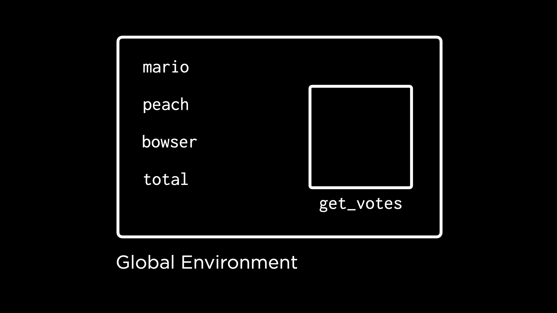
• Turns out all objects are defined within certain “environments.” One such environment is the “global” environment. The global environment is home to objects you define in the R console or outside of a function body—objects like mario, bowser, and peach. By default, RStudio’s environment pane shows you objects defined in the global environment.

  

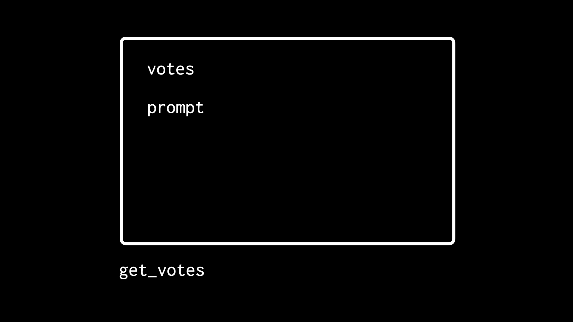
• The get_votes function is also an object defined in the global environment. What’s unique, though, is that get_votes is also a kind of environment in itself! As you’ve seen, within the definition of get_votes, you can define other objects, like votes and prompt.

  

• The environment of get_votes is not the global environment. While writing code that operates in the global environment, objects in this environment are not accessible.
• The environment(s) in which an object is available is known as its “scope.”

Checking Input

• One of the challenges consistently facing programmers is the bad behavior of users. That is, we should expect, as programmers, that users will not always do what we want. For instance, what if a user provides a string of text instead of numbers for votes?

• We can improve our program to catch incorrect values that are entered:

  # Demonstrates anticipating invalid input
  
  get_votes <- function(prompt = "Enter votes: ") {
    votes <- as.integer(readline(prompt))
    if (is.na(votes)) {
      return(0)
    } else {
      return(votes)
    }
  }
  
  mario <- get_votes("Mario: ")
  peach <- get_votes("Peach: ")
  bowser <- get_votes("Bowser: ")
  
  total <- sum(mario, peach, bowser)
  cat("Total votes:", total)
  

  Notice how get_votes will return a 0 if the value for votes is NA. Otherwise, get_votes will return the value provided by the user.

• While this program works, it still provides warnings, which we may not want the user to see. We can suppress warnings as follows:

  # Demonstrates anticipating invalid input
  
  get_votes <- function(prompt = "Enter votes: ") {
    votes <- suppressWarnings(as.integer(readline(prompt)))
    if (is.na(votes)) {
      return(0)
    } else {
      return(votes)
    }
  }
  
  mario <- get_votes("Mario: ")
  peach <- get_votes("Peach: ")
  bowser <- get_votes("Bowser: ")
  
  total <- sum(mario, peach, bowser)
  cat("Total votes:", total)
  

  Notice how warnings are now suppressed when this code is run.

• This program can be further improved by using ifelse. Consider the following:

  # Demonstrates ifelse as last evaluated expression
  
  get_votes <- function(prompt = "Enter votes: ") {
    votes <- as.integer(readline(prompt))
    ifelse(is.na(votes), 0, votes)
  }
  
  mario <- get_votes("Mario: ")
  peach <- get_votes("Peach: ")
  bowser <- get_votes("Bowser: ")
  
  total <- sum(mario, peach, bowser)
  cat("Total votes:", total)
  

  Notice that the first value of ifelse is a logical expression to be tested. The second value, 0, is what will be returned if the first value is.na(votes) evaluates to TRUE. Finally, the third value, votes, is provided if the first value evaluates to FALSE.

• We have now discovered our first fundamental ways of checking user input.

• As we did prior, we can suppress warnings:

  # Demonstrates suppressWarnings
  
  get_votes <- function(prompt = "Enter votes: ") {
    votes <- suppressWarnings(as.integer(readline(prompt)))
    ifelse(is.na(votes), 0, votes)
  }
  
  mario <- get_votes("Mario: ")
  peach <- get_votes("Peach: ")
  bowser <- get_votes("Bowser: ")
  
  total <- sum(mario, peach, bowser)
  cat("Total votes:", total)
  

  Notice how warnings are suppressed.

Loops

• One significant improvement we may desire for our program is the ability to repeatedly prompt the user when they make an error.
• To learn more about loops, let’s enlist the help of the CS50 Duck Debugger! Quack!

• Consider the following code:

  # Demonstrates a duck quacking 3 times
  
  cat("quack!\n")
  cat("quack!\n")
  cat("quack!\n")
  

  Notice how this code will output quack three times. However, it’s quite inefficient! We are repeating the same line of code three times.

• We could attempt to improve this code using a repeat loop as follows:

  # Demonstrates duck quacking in an infinite loop
  
  repeat {
    cat("quack!\n")
  }
  

  Notice how our duck quacks multiple times, but forever. The duck is going to get very tired!

• One of the ways we can implement a loop is by utilizing break and next. Such a loop will repeat a number of times by using a counter.

  # Demonstrates quacking 3 times with repeat
  
  i <- 3
  repeat {
    cat("quack!\n")
    i <- i - 1
    if (i == 0) {
      break
    } else {
      next
    }
  }
  

  Notice how the value of i is set to 3. Then each time a quack! occurs, i is reduced by a value of 1. When 0 is reached, the loop will break. Otherwise (or else), this loop will continue with next.

• In the end, next is not required. The loop will automatically continue without the next statement. We can remove this statement as follows:

  # Demonstrates removing extraneous next keyword
  
  i <- 3
  repeat {
    cat("quack!\n")
    i <- i - 1
    if (i == 0) {
      break
    }
  }
  

  Notice how the loop will break when i is equal to 0. However, next has been removed. The loop will still function.

• Another type of loop at our disposal is called a while loop. Such a loop will continue as long as a certain condition has not been met. Consider the following code:

  # Demonstrates a while loop, counting down
  
  i <- 3
  while (i != 0) {
    cat("quack!\n")
    i <- i - 1
  }
  

  Notice how this loop will run while the value of i != 0 is true.

• Another type of loop is called a for loop that allows us to repeat based upon a list or vector of values:

  # Demonstrates a for loop
  
  for (i in c(1, 2, 3)) {
    cat("quack!\n")
  }
  

  Notice how a for loop starts the value of i at 1, running the code inside of it. Then, it will set the value of i to two and run. Finally, it will set i to 3 and run. Thus, the code within the loop runs three times.

• We can simplify our code by counting 1, 2, and 3 using the range 1:3 (one through three).

  # Demonstrates a for loop with syntactic sugar
  
  for (i in 1:3) {
    cat("quack!\n")
  }
  

  Notice how the code i in 1:3 accomplishes the same task as the code presented in the prior example.

Using Loops

• We can use our newly-learned abilities in loops in our counting of votes for Mario and friends. Consider the following code that utilizes a repeat loop:

  # Demonstrates reprompting the user for valid input
  
  get_votes <- function(prompt = "Enter votes: ") {
    repeat {
      votes <- suppressWarnings(as.integer(readline(prompt)))
      if (!is.na(votes)) {
        break
      }
    }
    return(votes)
  }
  
  mario <- get_votes("Mario: ")
  peach <- get_votes("Peach: ")
  bowser <- get_votes("Bowser: ")
  
  total <- sum(mario, peach, bowser)
  cat("Total votes:", total)
  

  Notice that the user will be reprompted until the value provided is not NA.

• We can further improve our code as follows:

  # Demonstrates tightening return
  
  get_votes <- function(prompt = "Enter votes: ") {
    repeat {
      votes <- suppressWarnings(as.integer(readline(prompt)))
      if (!is.na(votes)) {
        return(votes)
      }
    }
  }
  
  mario <- get_votes("Mario: ")
  peach <- get_votes("Peach: ")
  bowser <- get_votes("Bowser: ")
  
  total <- sum(mario, peach, bowser)
  cat("Total votes:", total)
  

  Notice how the return(votes) clause is put in the place of break. The same functionality remains for this function, but the code is more brief.

• Now, using our knowledge of for loops, we can improve our code that is repeated for Mario and friends:

  # Demonstrates prompting for input in a loop
  
  get_votes <- function(prompt = "Enter votes: ") {
    repeat {
      votes <- suppressWarnings(as.integer(readline(prompt)))
      if (!is.na(votes)) {
        return(votes)
      }
    }
  }
  
  for (name in c("Mario", "Peach", "Bowser")) {
    votes <- get_votes(paste0(name, ": "))
  }
  

  Notice how, instead of three separate lines to prompt the user for votes for each of the candidates, the for loop will run for the range of “Mario,” “Peach,” and “Bowser” to get the votes. The paste0 statement adds the : character to each of the prompts.

• As a final flourish, we can employ a loop to count the votes as we go:

  # Demonstrates prompting for input, tallying votes in a loop
  
  get_votes <- function(prompt = "Enter votes: ") {
    repeat {
      votes <- suppressWarnings(as.integer(readline(prompt)))
      if (!is.na(votes)) {
        return(votes)
      }
    }
  }
  
  total <- 0
  for (name in c("Mario", "Peach", "Bowser")) {
    votes <- get_votes(paste0(name, ": "))
    total <- total + votes
  }
  
  cat("Total votes:", total)
  

  Notice how the total number of votes is updated in each iteration of the for loop.

• Reflecting upon the above, you can see the fundamental programming power that loops provide you as a programmer.

Using Functions and Loops

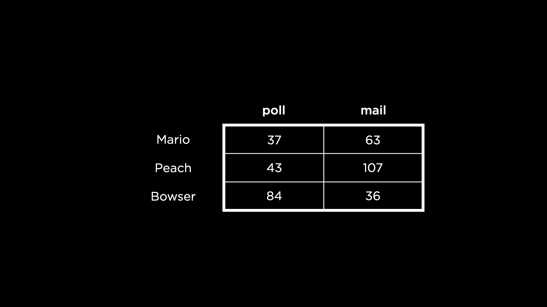
• Let’s return to a case that we discussed in a previous lecture, summing up candidates’ votes in a table like the below.

  

• Let’s now use our new abilities in loops and functions to create a better program.

• Perhaps our first goal should be to sum up the votes. Consider the following code:

  # Demonstrates summing votes for each candidate procedurally
  
  votes <- read.csv("votes.csv")
  
  total_votes <- c()
  for (candidate in rownames(votes)) {
    total_votes[candidate] <- sum(votes[candidate, ])
  }
  total_votes
  

  Notice how this for loop will iterate through each candidate presented in the votes data frame. Then the sum of the votes for the candidate will be stored in the total_votes vector. total_votes <- c() represents an empty vector that is later populated with data. total_votes[candidate] creates a new element within the vector total_votes, one for each candidate in each iteration of the loop.

• A second goal could be to sum the method by which each candidate received votes.

  # Demonstrates summing votes for each voting method procedurally
  
  votes <- read.csv("votes.csv")
  
  total_votes <- c()
  for (method in colnames(votes)) {
    total_votes[method] <- sum(votes[, method])
  }
  total_votes
  

  Notice how this for loop iterates through each method in the colnames (or column names).

Applying Functions

• The above program could be optimized further using a family of functions known as the apply functions.
• The apply functions allow you to apply (i.e., run) a function across elements of a data structure. For example, the apply function can apply a function across all rows or columns in a table of data.

• In the case of the votes table, we can use apply as follows to get the sum of all the rows:

  # Demonstrates summing votes for each candidate with apply
  
  votes <- read.csv("votes.csv")
  total_votes <- apply(votes, MARGIN = 1, FUN = sum)
  total_votes
  

  Notice how the sum function is applied to all of the rows using MARGIN = 1. Had we put MARGIN = 2, the sum function would have been applied to all of the columns.

• We can sum each column as follows:

  # Demonstrates summing votes for each voting method with apply
  
  votes <- read.csv("votes.csv")
  total_votes <- apply(votes, MARGIN = 2, FUN = sum)
  total_votes
  

  Notice how MARGIN = 2.

Summing Up

In this lesson, you learned how to represent data in R. Specifically, you learned…

• Defining Functions
• Scope
• Checking Input
• Loops
• Using Loops
• Using Functions and Loops
• Applying Functions

See you next time when we discuss how to clean up our data.