Lecture 3

• Searching
  • Searching Unsorted Data
  • Binary Searching
• Efficiency
• Sorting
  • Bubble Sort
  • Selection Sort
  • Merge Sort
• Memory
• Data Structures
  • Arrays
  • Linked Lists
  • Binary Search Trees
  • Hash Tables
• Python

Searching

Searching Unsorted Data

• Each of these boxes (numbered from 0 through 6) has a number in it. We want to find the number 50.

  0	1	2	3	4	5	6
  X	X	X	X	X	X	X

• At each step, we might open the first unopened box and look inside until we find the number 50.

  0	1	2	3	4	5	6
  X	X	X	X	X	X	X
  15	X	X	X	X	X	X
  15	23	X	X	X	X	X
  15	23	16	X	X	X	X
  15	23	16	8	X	X	X
  15	23	16	8	42	X	X
  15	23	16	8	42	50	X

• We found the number 50 after looking at n - 1 boxes, where n is the total number of boxes we have. Essentially, we looked at roughly n boxes.

Binary Searching

• Each of these boxes has a number behind it. The numbers are sorted now, and we want to find the number 50.

  0	1	2	3	4	5	6
  X	X	X	X	X	X	X

• We’d like to use the divide and conquer strategy that we previously used with our phone book.

• First, we’ll go to the middle box and look at the number.

  • Since these numbers are back to back to back, we can mathematically determine which index to look at. Then, the computer can jump to that index in constant time.

  • There are 7 boxes, so the middle number must be at index 7/2 = 3.5, rounding down, gives us 3.

  • Remembering that we start with the 0th index, we open the box at the 3rd index.

    0	1	2	3	4	5	6
    X	X	X	16	X	X	X

• Next, we’ll compare the number 16 to what we’re searching for: 50. 50 is larger, so we know that 50 cannot be located in any box before 16.

• We’ll now search the remainder of the boxes in a similar manner. We’ll go to the middle box and look at the number.

  • There are 3 boxes, so the middle number must be at index 3/2 = 1.5, rounding down, gives us 1.

  • We open the box at the 1st index.

    0	1	2	3	4	5	6
    X	X	X	16	X	42	X

• We compare the number 42 to what we’re searching for: 50. 50 is larger, so we know that 50 cannot be located in any box before 42.

• We search the remainder of the boxes.

  • There is only 1 box remaining, so the “middle” number is at index 1/2 = 0.5, rounding down, gives us 0.

  • We open the box at the 0th index.

    0	1	2	3	4	5	6
    X	X	X	16	X	42	50

• Finally, we compare 50 to what we’re searching for: 50. We’ve found it!

• This arrangement, having data stored back to back to back, is known as an array.

• Note that this only took us 3 steps. Like dividing and conquering the phone book, this algorithm also has log(n) efficiency.

Efficiency

• When discussing upper bounds on how much time an algorithm takes, we say that an algorithm has a big O of some formula.

  • Some formulas, where n is a variable that represents the size of the problem, include

    • n²

    • nlog(n)

    • n

    • log(n)

    • 1

  • For example, for linear search, when we’re searching boxes left to right or searching from the beginning of the phone book to the end, in the worst case, it might take as many as n steps to find the 50 or Mike Smith. Thus, we would say that the linear search algorithm is O(n).

  • For binary search, note that we are able to “remove” half the list each time. Thus, if we double the size of the input, it only requires one additional step. The binary search algorithm is O(log n).

• When discussing lower bounds on how much time an algorithm takes, we say that algorithm is Ω of some formula.

  • Using the previous example, if the first few boxes we look at has 50 in it or if one of the first few entries in the phone book is Mike Smith, then the number of steps we take does not depend on n. In this case, the linear search algorithm is Ω(1).

  • The binary search algorithm is Ω(1) as well.

• When the upper bound and lower bound are the same, we can say that the algorithm is ϴ of some formula.

Sorting

• It was more efficient searching a sorted list than an unsorted list. Now, we’ll discuss how we might sort a list.

Bubble Sort

• In bubble sort, the larger numbers bubble to the top during the sorting process.

• Let’s start with these unsorted numbers. Their indexes are shown above. We wish to sort them in ascending order.

  0	1	2	3	4	5	6	7
  2	1	6	5	4	3	8	7

  • First Pass

    • Looking at the first two numbers (0th and 1st index), 2 > 1, so we swap them.

      0	1	2	3	4	5	6	7
      1	2	6	5	4	3	8	7

    • Next, looking at 2 and 6 (1st and 2nd index), we note that they are in the right order.

    • Looking at 5 and 6 (2nd and 3rd index), we note that 6 > 5, so we swap them.

      0	1	2	3	4	5	6	7
      1	2	5	6	4	3	8	7

    • Next, looking at 6 and 4 (3rd and 4th index), we note that 6 > 4, so we swap them.

      0	1	2	3	4	5	6	7
      1	2	5	4	6	3	8	7

    • Next, looking at 6 and 3 (4th and 5th index), we note that 6 > 3, so we swap them.

      0	1	2	3	4	5	6	7
      1	2	5	4	3	6	8	7

    • Next, looking at 6 and 8 (5th and 6th index), we note that they are in the right order.

      0	1	2	3	4	5	6	7
      1	2	5	4	3	6	8	7

    • Next, looking at 8 and 7 (6th and 7th index), we note that 8 > 7, so we swap them.

      0	1	2	3	4	5	6	7
      1	2	5	4	3	6	7	8

  • Second Pass

    • We follow the same steps as above, comparing the adjacent numbers.

    • After the second pass, we get

      0	1	2	3	4	5	6	7
      1	2	4	3	5	6	7	8

  • We can continue with the passes: after each pass, the largest unsorted number is placed in its sorted position. After n passes, we can guarantee that all n elements are sorted.

• The pseudocode we might write is:

    repeat until no swaps
        for i from 0 to n-2
            if i'th and i+1'th elements out of order
                swap them
  

  • i is an integer that represents an index
  • Since we are comparing the i‘th and i+1‘th element, we only need to go up to n-2 for i. Then, we swap the two elements if they’re out of order.

• We are making n-1 comparisons, or roughly n comparisons, for each pass. Additionally, we make roughly n passes. Multiplying, this algorithm is on the order of n².

• With each step, we are improving the sortedness of the data. Essentially, we are solving local problems to achieve a global result.

Selection Sort

• In selection sort, in each pass, we select the smallest number.

• Let’s start with these unsorted numbers. We wish to sort them in ascending order.

  0	1	2	3	4	5	6	7
  2	3	1	5	8	7	6	4

  • First pass:

    • We look at the first unsorted number, which is 2. Now, we look at the rest of the list.

      • 3 is greater than 2, so 2 is still the smallest.
      • 1 is less than 2, so 1 is now the smallest.
      • 5 is greater than 1, so 1 is still the smallest.
      • 8 is greater than 1, so 1 is still the smallest.
      • …
      • 4 is greater than 1, so 1 is still the smallest.

    • Now, we swap the 1 with the first unsorted number, or 2. We get this list:

      0	1	2	3	4	5	6	7
      1	3	2	5	8	7	6	4

  • Second pass:

    • We look at the first unsorted number, which is 3. Now, we look at the rest of the list.

      • 2 is less than 3, so 2 is now the smallest.
      • 5 is greater than 2, so 2 is still the smallest.
      • 8 is greater than 2, so 2 is still the smallest.
      • …
      • 4 is greater than 2, so 2 is still the smallest.

    • Now, we swap the 2 with the first unsorted number, or 3. We get this list:

      0	1	2	3	4	5	6	7
      1	2	3	5	8	7	6	4

  • Third pass:

    • We proceed similarly. After the third pass, we find that 3 is the smallest, and it is in the correct position.

  • Fourth pass:

    • After the fourth pass, we find that 4 is the smallest, and we swap 5 with 4.

      0	1	2	3	4	5	6	7
      1	2	3	4	8	7	6	5

  • Fifth pass:

    • After the fifth pass, we find that 5 is the smallest, and we swap 8 with 5.

      0	1	2	3	4	5	6	7
      1	2	3	4	5	7	6	8

  • Sixth pass:

    • After the sixth pass, we find that 6 is the smallest, and we swap 7 with 6.

      0	1	2	3	4	5	6	7
      1	2	3	4	5	6	7	8

  • Seventh pass:

    • After the seventh pass, we find that 7 is the smallest, and it is in the correct position.

      0	1	2	3	4	5	6	7
      1	2	3	4	5	6	7	8

• The pseudocode we might write is:

    for i from 0 to n-1
        find smallest element between i'th and n-1'th
        swap smallest with i'th element
  

• Note that the amount left to be sorted steadily decreases. For the first pass, we look through n elements. For the second pass, we look through n-1 elements. This continues until we only have 1 element left. Adding these, we get

  n + n-1 + n-2 + ... + 1 = n(n - 1)/2 = n^2/2 - n/2.

• We can ignore the lower level terms, and this algorithm is on the order of n².

• Why can we ignore the lower level terms? These terms play an insignificant role once n is large.

  • For example, if n = 1000000, then n²/2 - n/2 = 1000000²/2 - 1000000/2.

  • This is equivalent to 500000000000 - 500000 = 499999500000. This value is pretty close to 1000000²/2 or 500000000000.

Merge Sort

• Instead of sorting the entire list at once, we can implement a divide and conquer strategy.

• When we have an unsorted list, we will

  1. Sort the left half.
  2. Sort the right half.
  3. Interweave the two lists together.

• For step 1, when sorting the left half, we can apply the same algorithm. We sort the left half of the left half, then the right half of the left half, and then we merge them together.

• If we continue to halve and halve, we’ll end up with one element as the left half and one element as the right half. We no longer have to do steps 1 and 2 since the halves are already sorted, but we do have to interweave these two in order to merge them.

• Merge sort takes less time than the previous two sorts, but there is a trade-off. Merge sort takes twice as much space, as it requires additional space to sort the halves before interweaving the halves.

Memory

• Computers store data in RAM or Random Access Memory. The term “Random” in this case refers to a computer’s ability to jump in constant time to a specific byte.

• Pictured is a memory chip on a RAM stick. The grid is an artist’s rendition of how we can number each of the bytes in the chip.

  

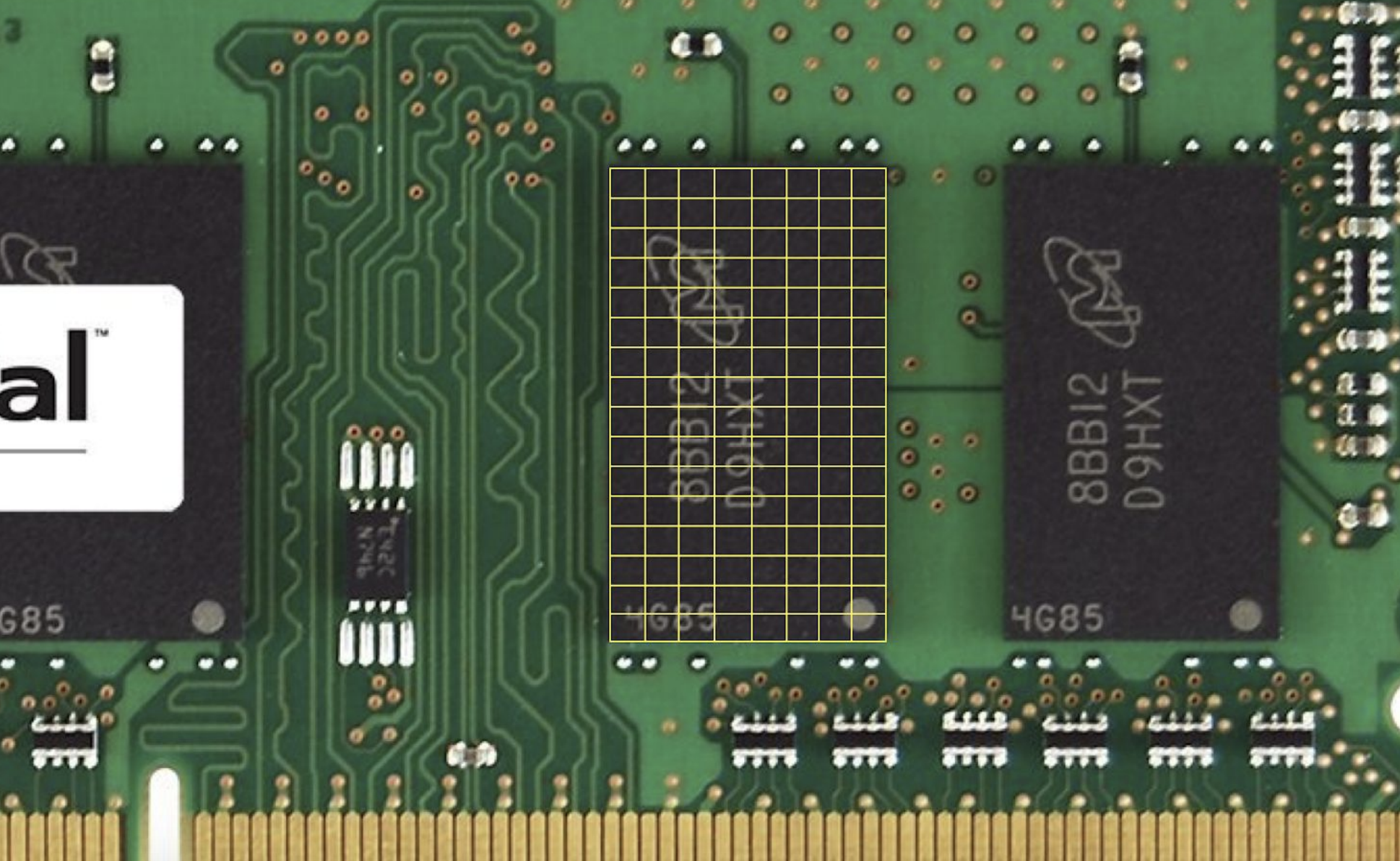
• When we store a float, we’re asking the computer for 32 bits. Bytes to the left or right of the allocated memory might already be in use, so we can’t use more than 32 bits for this float. This leads to floating point imprecision, a topic from the previous week.

Data Structures

Arrays

• All of the previously mentioned algorithms assume that the values are stored in an array.

• When we store numbers in an array, each value is back to back, so we can use arithmetic to get an index. Then, we can instantly jump to that address. This gives us random access, which is constant time.

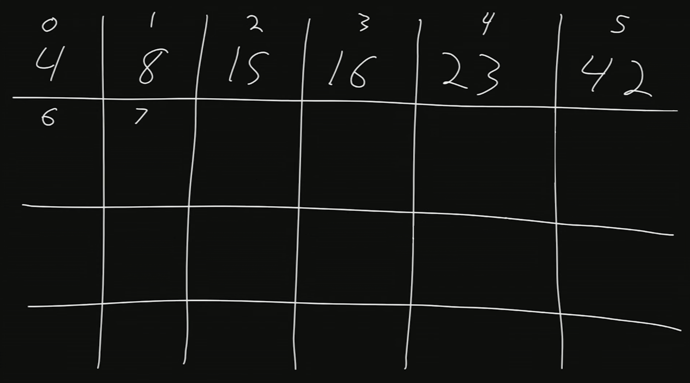
• Suppose we want to store six values in memory. We then ask our operating system for just enough bytes for six numbers. The indexes are numbered 0 through 7.

  

  • What if we wanted to add the number 50?

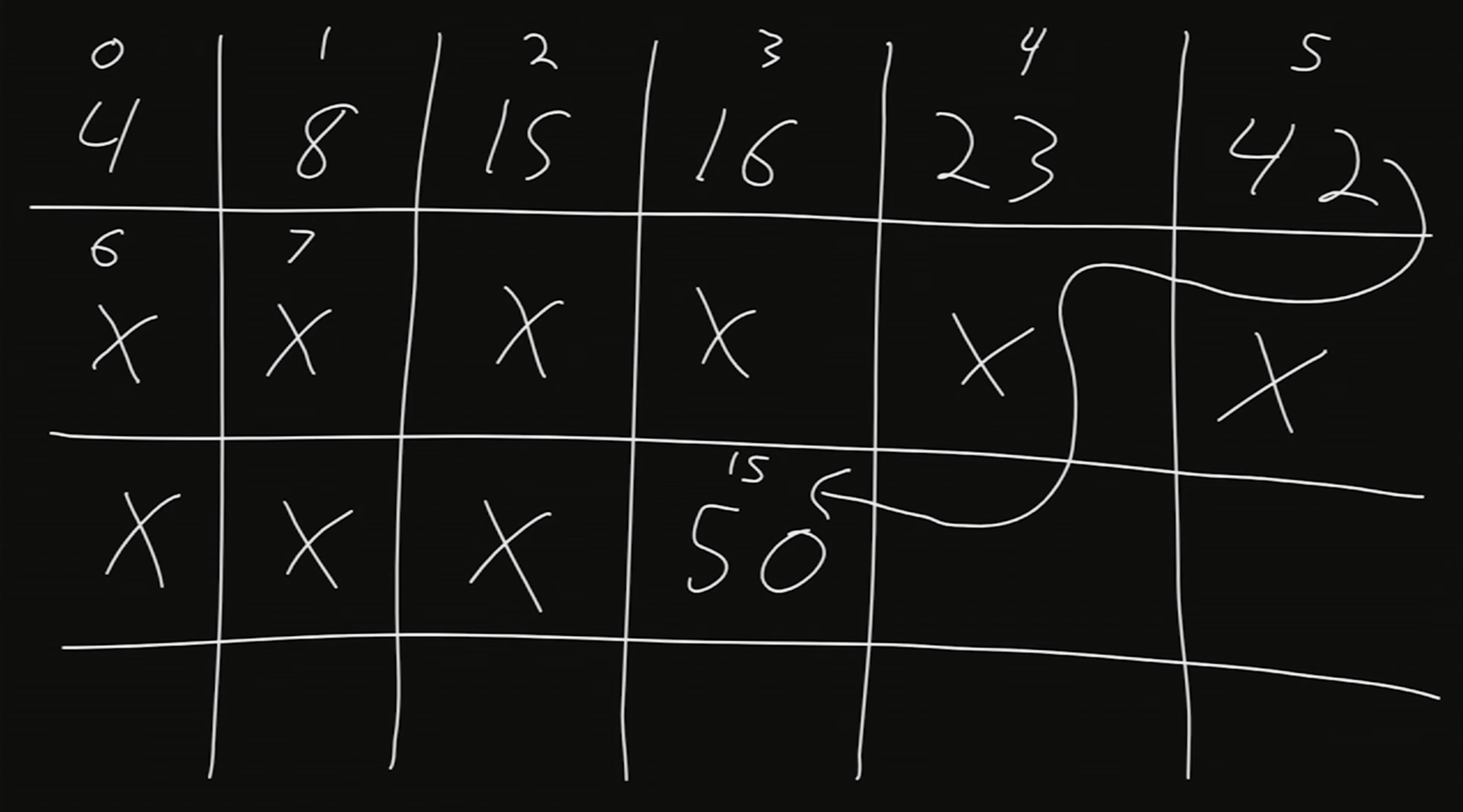
  • Since we only asked our operating system for enough bytes for six numbers, the operating system might have already allocated the memory from 6 and beyond to some other aspect of our program.

  • For a temporary fix, we could’ve just asked the operating system for enough space for 7 or 8 or even 100 values.

    • In this case, we’re asking for more memory than we actually need. Then, the computer has less space for other programs to store and run.

  • We could also just add 50 where there is free space. Let’s say at index 15, we have space to store 50. Let’s draw an arrow to denote that after 42 comes 50.

    

    • The equivalent to drawing an arrow is to store the address of the number 50 alongside 42. This way, once we get to 42, we’ll note that we should go to index 15.

    • We don’t have enough space at index 5 to store both 42 and the address. Instead, we’ll take note of this idea of storing addresses.

Linked Lists

• A linked list allows us to store and remove values by linking the values together.

• 

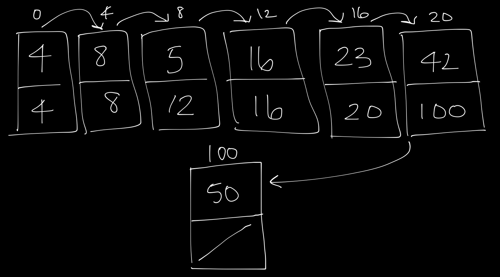
  • In each node, or box drawn here, we store a value (data) and the address of the next value.

  • For example, the first node contains the value 4. To find the next value, we go to the address stored, which is 4. Then, we go to the 4th index, which has the value 8.

  • As another example, assume we’re at the index 20. It has value 42. To go to the next value, we go to the address indicated on this node, of index 100. We find that at index 100, we have the value 50.

• To remove a node, we can simply snip it out and redirect an arrow, thereby changing an address.

• To add a node, we can store it somewhere and update the address at index 100 to point to the new node.

• We’re now able to add and remove values, but we no longer have random access. To search through a linked list, we must traverse in linear time from the first element to the last.

• Additionally, we are using twice as much space as an array since we also have to store the next node’s address.

Binary Search Trees

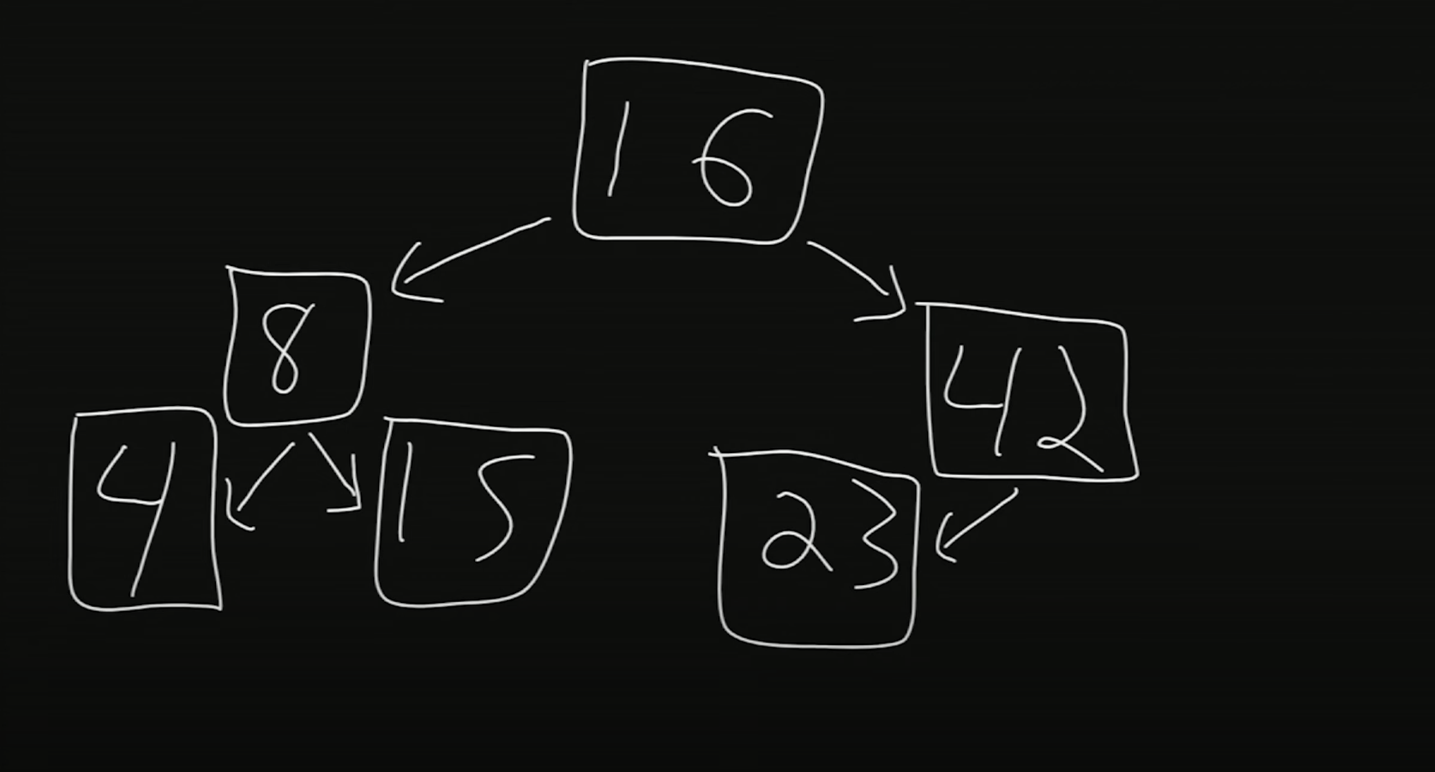
• In a binary search tree, each node has two children (hence binary), one child less than it and one child greater than it.

• 

  • 16 is the root of this tree.

  • To the left of 16 is its left child, and to the right of 16 is its right child.

  • Within this tree, we also have many subtrees. The children of 16 are subtrees themselves; for example, rooted at 8 is a child called 4 and a child called 15.

  • Note that for each node N, its left child is less than N and its right child is greater than N.

  • Let’s look for the number 15 in this structure. We’ll start at 16, the root node. 15 is less than 16, so we’ll go to the left child. 15 is greater than 8, so we go to the right child. And we’ve found 15!

    • In searching this binary search tree, we looked at less nodes than we would in a linked list. By having a 2 dimensional data structure, we were able to create more organization.

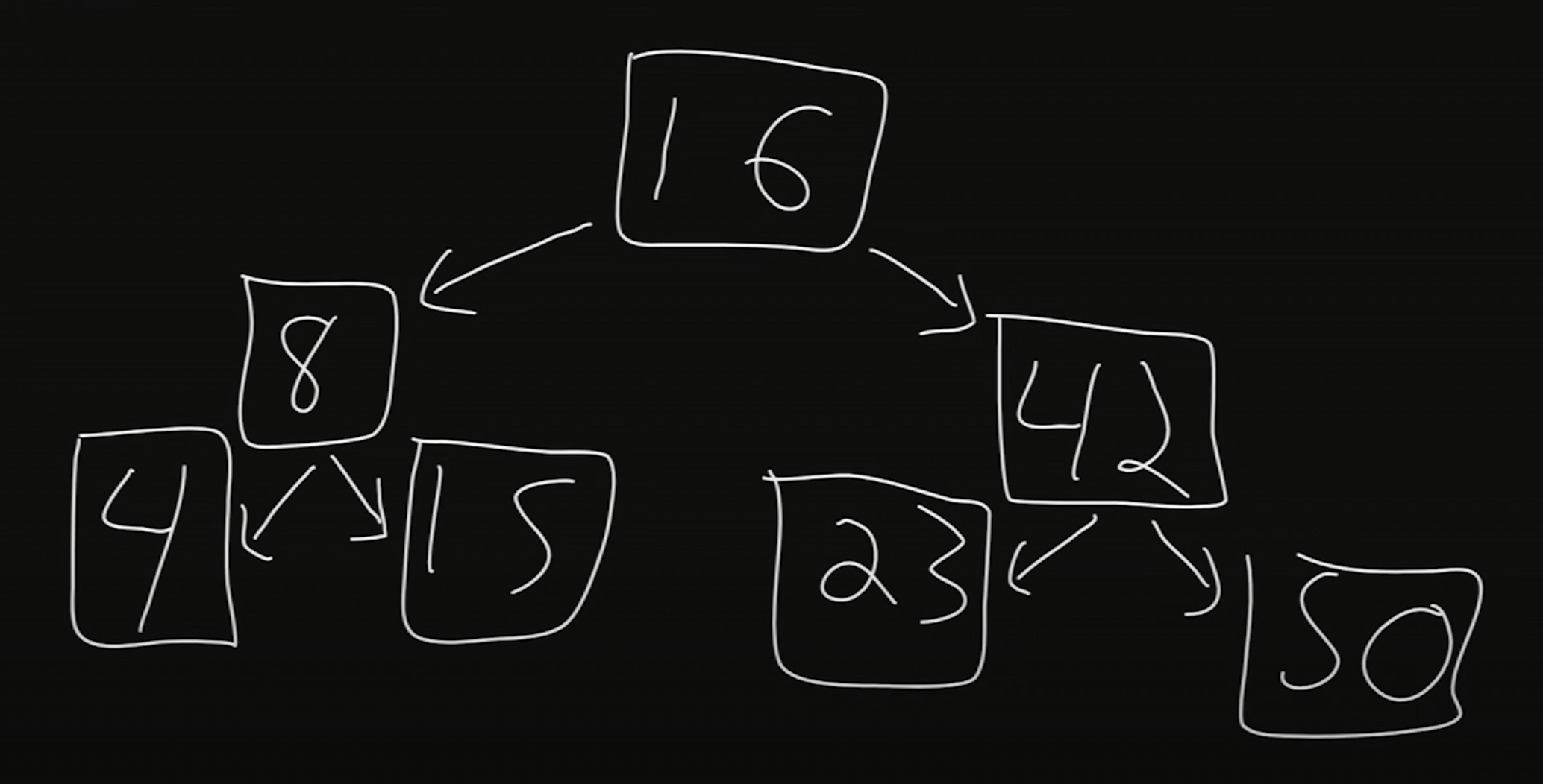
  • We can also easily modify the size of the binary search tree. Suppose we wanted to add the number 50. Starting from the root, we note that 50 is greater than 16, so we go to the right child. 50 is also greater than 42, and 42 does not have a right child yet. Thus, we insert 50 as the right child of 42.

    

• Binary trees can become unbalanced if we just keep adding larger and larger values. There exist more complex algorithms that are able to re-balance the tree after adding values.

• With a binary search tree, we can add and remove values and search quickly. However, the tradeoff is requiring more space, as 2 additional chunks of memory are required to store the 2 children.

Hash Tables

• Hash tables have constant search time. Let’s look at an example.

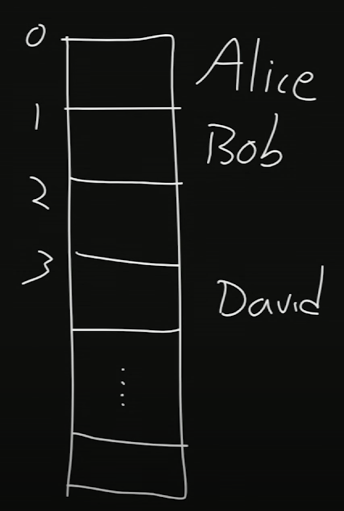
• Here, we have an array. Alice is stored at index 0, Bob is stored at index 1, and David is stored at index 3.

  

  • A hash function takes some value as input and returns an index where we store the value. The particular hash function we’re using here looks at the first letter of each string. An A at the first letter will map to the 0th index, a B at the first letter will map to the 1st index, and so on.

    • The function in this case, takes the ASCII value of the first letter and subtracts 65, which is the ASCII value for A.

  • Inserting these names is thus constant time, as hashing is constant time and we can get to that index via random access.

• When we add Doug, we’ll note that David is already in index 3 of this array. This is considered a collision, where multiple inputs map to the same output.

• To store both values, we’ll use a linked list. It might look like this:

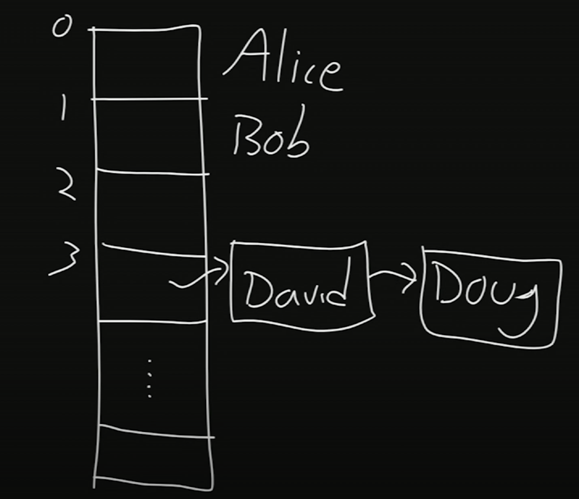
• A hash table approximates constant time—for a good hash function, we’ll have very few collisions, meaning we won’t have to traverse through linked lists to search for, add, or delete a value.

Python

• Certain data types in Python are reminiscent of the data structures here.

• In Python, the dict type stands for dictionary. This is essentially a hash table.

  • The indexes in this case are words.

  • Via these indexes or words, we can return a value.

• In Python, the list type is an array that we can change the size of, similar to a linked list.