Lecture 3
Last week
- We learned about tools to solve problems, or bugs, in our code. In particular, we discovered how to use a debugger, a tool that allows us to step slowly through our code and look at values in memory while our program is running.
- Another powerful, if less technical, tool is rubber duck debugging, where we try to explain what we’re trying to do to a rubber duck (or some other object), and in the process realize the problem (and hopefully solution!) on our own.
- We looked at memory, visualizing bytes in a grid and storing values in each box, or byte, with variables and arrays.
Searching
- It turns out that, with arrays, a computer can’t look at all of the elements at once. Instead, a computer can only to look at them one at a time, though the order can be arbitrary. (Recall in Week 0, David could only look at one page at a time in a phone book, whether he flipped through in order or in a more sophisticated way.)
- Searching is how we solve the problem of finding a particular value. A simple case might have an input of some array of values, and the output might simply be a
bool, whether or not a particular value is in the array. - Today we’ll look at algorithms for searching. To discuss them, we’ll consider running time, or how long an algorithm takes to run given some size of input.
Big \(O\)
- In week 0, we saw different types of algorithms and their running times:
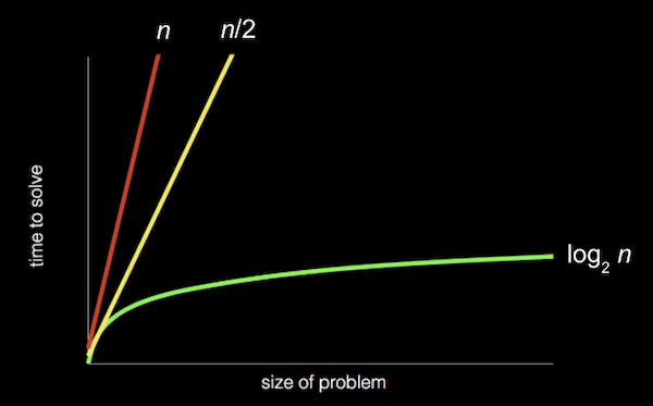
- Recall that the red line is searching linearly, one page at a time; the yellow line is searching two pages at a time; and the green line is searching logarithmically, dividing the problem in half each time.
- And these running times are for the worst case, or the case where the value takes the longest to find (on the last page, as opposed to the first page).
- The more formal way to describe each of these running times is with big \(O\) notation, which we can think of as “on the order of”. For example, if our algorithm is linear search, it will take approximately \(O(n)\) steps, read as “big \(O\) of \(n\)” or “on the order of \(n\)”. In fact, even an algorithm that looks at two items at a time and takes \(n/2\) steps has \(O(n)\). This is because, as \(n\) gets bigger and bigger, only the dominant factor, or largest term, \(n\), matters. In the chart above, if we zoomed out and changed the units on our axes, we would see the red and yellow lines end up very close together.
- A logarithmic running time is \(O(\log n)\), no matter what the base is, since this is just an approximation of what fundamentally happens to running time if \(n\) is very large.
- There are some common running times:
- \(O(n^2)\)
- \(O(n \log n)\)
- \(O(n)\)
- (searching one page at a time, in order)
- \(O(\log n)\)
- (dividing the phone book in half each time)
- \(O(1)\)
- An algorithm that takes a constant number of steps, regardless of how big the problem is.
- Computer scientists might also use big \(Ω\), big Omega notation, which is the lower bound of number of steps for our algorithm. Big \(O\) is the upper bound of number of steps, or the worst case.
- And we have a similar set of the most common big Ω running times:
- \(\Omega(n^2)\)
- \(\Omega(n \log n)\)
- \(\Omega(n)\)
- \(\Omega(\log n)\)
- \(\Omega(1)\)
- (searching in a phone book, since we might find our name on the first page we check)
Linear search, binary search
- On stage, we have a few prop doors, with numbers hidden behind them. Since a computer can only look at one element in an array at a time, we can only open one door at a time as well.
- If we want to look for the number zero, for example, we would have to open one door at a time, and if we didn’t know anything about the numbers behind the doors, the simplest algorithm would be going from left to right.
- So, we might write pseudocode for linear search with:
For i from 0 to n–1 If number behind i'th door Return true Return false- We label each of
ndoors from0ton–1, and check each of them in order. - “Return false” is outside the for loop, since we only want to do that after we’ve looked behind all the doors.
- The big \(O\) running time for this algorithm would be \(O(n)\), and the lower bound, big Omega, would be \(\Omega(1)\).
- We label each of
- If we know that the numbers behind the doors are sorted, then we can start in the middle, and find our value more efficiently.
- For binary search, our algorithm might look like:
If no doors Return false If number behind middle door Return true Else if number < middle door Search left half Else if number > middle door Search right half- The upper bound for binary search is \(O(\log n)\), and the lower bound also \(\Omega(1)\), if the number we’re looking for is in the middle, where we happen to start.
- With 64 light bulbs, we notice that linear search takes much longer than binary search, which only takes a few steps.
- We turned off the light bulbs at a frequency of one hertz, or cycle per second, and a processor’s speed might be measured in gigahertz, or billions of operations per second.
Searching with code
- Let’s take a look at
numbers.c:#include <cs50.h> #include <stdio.h> int main(void) { int numbers[] = {4, 6, 8, 2, 7, 5, 0}; for (int i = 0; i < 7; i++) { if (numbers[i] == 0) { printf("Found\n"); return 0; } } printf("Not found\n"); return 1; }- Here we initialize an array with some values in curly braces, and we check the items in the array one at a time, in order, to see if they’re equal to zero (what we were originally looking for behind the doors on stage).
- If we find the value of zero, we return an exit code of 0 (to indicate success). Otherwise, after our for loop, we return 1 (to indicate failure).
- We can do the same for names:
#include <cs50.h> #include <stdio.h> #include <string.h> int main(void) { string names[] = {"Bill", "Charlie", "Fred", "George", "Ginny", "Percy", "Ron"}; for (int i = 0; i < 7; i++) { if (strcmp(names[i], "Ron") == 0) { printf("Found\n"); return 0; } } printf("Not found\n"); return 1; }- Note that
namesis a sorted array of strings. - We can’t compare strings directly in C, since they’re not a simple data type but rather an array of many characters. Luckily, the
stringlibrary has astrcmp(“string compare”) function which compares strings for us, one character at a time, and returns0if they’re the same. - If we only check for
strcmp(names[i], "Ron")and notstrcmp(names[i], "Ron") == 0, then we’ll printFoundeven if the name isn’t found. This is becausestrcmpreturns a value that isn’t0if two strings don’t match, and any nonzero value is equivalent to true in a condition.
- Note that
Structs
- If we wanted to implement a program that searches a phone book, we might want a data type for a “person”, with their name and phone number.
- It turns out in C that we can define our own data type, or data structure, with a struct in the following syntax:
typedef struct { string name; string number; } person;- We use
stringfor thenumber, since we want to include symbols and formatting, like plus signs or hyphens. - Our struct contains other data types inside it.
- We use
- Let’s try to implement our phone book without structs first:
#include <cs50.h> #include <stdio.h> #include <string.h> int main(void) { string names[] = {"Brian", "David"}; string numbers[] = {"+1-617-495-1000", "+1-949-468-2750"}; for (int i = 0; i < 2; i++) { if (strcmp(names[i], "David") == 0) { printf("Found %s\n", numbers[i]); return 0; } } printf("Not found\n"); return 1; }- We’ll need to be careful to make sure that the firstname in
namesmatches the first number innumbers, and so on. - If the name at a certain index
iin thenamesarray matches who we’re looking for, we can return the phone number in thenumbersarray at the same index.
- We’ll need to be careful to make sure that the firstname in
- With structs, we can be a little more confident that we won’t have human errors in our program:
#include <cs50.h> #include <stdio.h> #include <string.h> typedef struct { string name; string number; } person; int main(void) { person people[2]; people[0].name = "Brian"; people[0].number = "+1-617-495-1000"; people[1].name = "David"; people[1].number = "+1-949-468-2750"; for (int i = 0; i < 2; i++) { if (strcmp(people[i].name, "David") == 0) { printf("Found %s\n", people[i].number); return 0; } } printf("Not found\n"); return 1; }- We create an array of the
personstruct type, and name itpeople(as inint numbers[], though we could name it arbitrarily, like any other variable). We set the values for each field, or variable, inside eachpersonstruct, using the dot operator,.. - In our loop, we can now be more certain that the
numbercorresponds to thenamesince they are from the samepersonstruct. - We can also improve the design of our program with a constant, like
const int NUMBER = 10;, and store our values not in our code but in a separate file or even a database, which we’ll soon see.
- We create an array of the
- Soon too, we’ll write our own header files with definitions for structs, so they can be shared across different files for our program.
Sorting
- If our input is an unsorted list of numbers, there are many algorithms we could use to produce an output of a sorted list, where all the elements are in order.
- With a sorted list, we can use binary search for efficiency, but it might take more time to write a sorting algorithm for that efficiency, so sometimes we’ll encounter the tradeoff of time it takes a human to write a program compared to the time it takes a computer to run some algorithm. Other tradeoffs we’ll see might be time and complexity, or time and memory usage.
Selection sort
- Brian is backstage with a set of numbers on a shelf, in unsorted order:
6 3 8 5 2 7 4 1 - Taking some numbers and moving them to their right place, Brian sorts the numbers pretty quickly.
- Going step-by-step, Brian looks at each number in the list, remembering the smallest one we’ve seen so far. He gets to the end, and sees that 1 is the smallest, and he knows that must go at the beginning, so he’ll just swap it with the number at the beginning, 6:
6 3 8 5 2 7 4 1 – – 1 3 8 5 2 7 4 6 - Now Brian knows at least the first number is in the right place, so he can look for the smallest number among the rest, and swap it with the next unsorted number (now the second number):
1 3 8 5 2 7 4 6 – – 1 2 8 5 3 7 4 6 - And he repeats this again, swapping the next smallest, 3, with the 8:
1 2 8 5 3 7 4 6 - - 1 2 3 5 8 7 4 6 - After a few more swaps, we end up with a sorted list.
- This algorithm is called selection sort, and we can be a bit more specific with some pseudocode:
For i from 0 to n–1 Find smallest item between i'th item and last item Swap smallest item with i'th item- The first step in the loop is to look for the smallest item in the unsorted part of the list, which will be between the i’th item and last item, since we know we’ve sorted up to the “i-1’th” item.
- Then, we swap the smallest item with the i’th item, which makes everything up to the item at i sorted.
- We look at a visualization online with animations for how the elements move for insertion sort.
- For this algorithm, we were looking at roughly all \(n\) elements to find the smallest, and making \(n\) passes to sort all the elements.
- More formally, we can use some math formulas to show that the biggest factor is indeed \(n^2\). We started with having to look at all \(n\) elements, then only \(n - 1\), then \(n - 2\):
\(n + (n – 1) + (n – 2) + ... + 1\)
\(n(n + 1)/2\)
\((n^2 + n)/2\)
\(n^2/2 + n/2\)
\(O(n^2)\)
- Since \(n^2\) is the biggest, or dominant, factor, we can say that the algorithm has running time of \(O(n^2)\).
Bubble sort
- We can try a different algorithm, one where we swap pairs of numbers repeatedly, called bubble sort.
- Brian will look at the first two numbers, and swap them so they are in order:
6 3 8 5 2 7 4 1 – – 3 6 8 5 2 7 4 1 - The next pair,
6and8, are in order, so we don’t need to swap them. - The next pair,
8and5, need to be swapped:3 6 8 5 2 7 4 1 – – 3 6 5 8 2 7 4 1 - Brian continues until he reaches the end of the list:
3 6 5 2 8 7 4 1 – – 3 6 5 2 7 8 4 1 – – 3 6 5 2 7 4 8 1 – – 3 6 5 2 7 4 1 8 - - Our list isn’t sorted yet, but we’re slightly closer to the solution because the biggest value,
8, has been shifted all the way to the right. And other bigger numbers have also moved to the right, or “bubbled up”. - Brian will make another pass through the list:
3 6 5 2 7 4 1 8 – – 3 6 5 2 7 4 1 8 – – 3 5 6 2 7 4 1 8 – – 3 5 2 6 7 4 1 8 – – 3 5 2 6 7 4 1 8 – – 3 5 2 6 4 7 1 8 - – 3 5 2 6 4 1 7 8 - -- Note that we didn’t need to swap the 3 and 6, or the 6 and 7.
- But now, the next biggest value,
7, moved all the way to the right.
- Brian will repeat this process a few more times, and more and more of the list becomes sorted, until we have a fully sorted list.
- With selection sort, the best case with a sorted list would still take just as many steps as the worst case, since we only check for the smallest number with each pass.
- The pseudocode for bubble sort might look like:
Repeat until sorted For i from 0 to n–2 If i'th and i+1'th elements out of order Swap them- Since we are comparing the
i'thandi+1'thelement, we only need to go up to \(n – 2\) fori. Then, we swap the two elements if they’re out of order. - And we can stop as soon as the list is sorted, since we can just remember whether we made any swaps. If not, the list must be sorted already.
- Since we are comparing the
- To determine the running time for bubble sort, we have \(n – 1\) comparisons in the loop, and at most \(n – 1\) loops, so we get \(n^2 – 2n + 2\) steps total. But the largest factor, or dominant term, is again \(n^2\) as
ngets larger and larger, so we can say that bubble sort has \(O(n^2)\). So it turns out that fundamentally, insertion sort and bubble sort has the same upper bound for running time. - The lower bound for running time here would be \(\Omega(n)\), once we look at all the elements once.
- So our upper bounds for running time that we’ve seen are:
- \(O(n^2)\)
- selection sort, bubble sort
- \(O(n \log n)\)
- \(O(n)\)
- linear search
- \(O(\log n)\)
- binary search
- \(O(1)\)
- \(O(n^2)\)
- And for lower bounds:
- \(\Omega(n^2)\)
- selection sort
- \(\Omega(n \log n)\)
- \(\Omega(n)\)
- bubble sort
- \(\Omega(\log n)\)
- \(\Omega(1)\)
- linear search, binary search
- \(\Omega(n^2)\)
Recursion
- Recursion is the ability for a function to call itself. We haven’t seen this in code yet, but we’ve seen something in pseudocode in week 0 that we might be able to convert:
1  Pick up phone book
2  Open to middle of phone book
3  Look at page
4  If Smith is on page
5      Call Mike
6  Else if Smith is earlier in book
7      Open to middle of left half of book
8      Go back to line 3
9  Else if Smith is later in book
10     Open to middle of right half of book
11     Go back to line 3
12 Else
13     Quit
- Here, we’re using a loop-like instruction to go back to a particular line.
- We could instead just repeat our entire algorithm on the half of the book we have left:
1  Pick up phone book
2  Open to middle of phone book
3  Look at page
4  If Smith is on page
5      Call Mike
6  Else if Smith is earlier in book
7      Search left half of book
8
9  Else if Smith is later in book
10     Search right half of book
11
12 Else
13     Quit
- This seems like a cyclical process that will never end, but we’re actually changing the input to the function and dividing the problem in half each time, stopping once there’s no more book left.
- In week 1, too, we implemented a “pyramid” of blocks in the following shape:
# ## ### #### - But notice that a pyramid of height 4 is actually a pyramid of height 3, with an extra row of 4 blocks added on. And a pyramid of height 3 is a pyramid of height 2, with an extra row of 3 blocks. A pyramid of height 2 is a pyramid of height 1, with an extra row of 2 blocks. And finally, a pyramid of height 1 is just a single block.
- With this idea in mind, we can write a recursive function to draw a pyramid, a function that calls itself to draw a smaller pyramid before adding another row.
Merge sort
- We can take the idea of recusion to sorting, with another algorithm called merge sort. The pseudocode might look like:
If only one number Return Else Sort left half of number Sort right half of number Merge sorted halves - We’ll best see this in practice with two sorted lists:
3 5 6 8 | 1 2 4 7 - We’ll merge the two lists for a final sorted list by taking the smallest element at the front of each list, one at a time:
3 5 6 8 | _ 2 4 7 1 - The 1 on the right side is the smallest between 1 and 3, so we can start our sorted list with it.
3 5 6 8 | _ _ 4 7 1 2 - The next smallest number, between 2 and 3, is 2, so we use the 2.
_ 5 6 8 | _ _ 4 7

1 2 3
_ 5 6 8 | _ _ _ 7 1 2 3 4_ _ 6 8 | _ _ _ 7 1 2 3 4 5_ _ _ 8 | _ _ _ 7 1 2 3 4 5 6_ _ _ 8 | _ _ _ _ 1 2 3 4 5 6 7_ _ _ _ | _ _ _ _ 1 2 3 4 5 6 7 8- Now we have a completely sorted list.
- We’ve seen how the final line in our pseudocode can be implemented, and now we’ll see how the entire algorithm works:
If only one number Return Else Sort left half of number Sort right half of number Merge sorted halves - We start with another unsorted list:
6 3 8 5 2 7 4 1 - To start, we need to sort the left half first:
6 3 8 5 - Well, to sort that, we need to sort the left half of the left half first:
6 3 - Now both of these halves just have one item each, so they’re both sorted. We merge these two lists together, for a sorted list:
_ _ 8 5 2 7 4 1 3 6 - We’re back to sorting the right half of the left half, merging them together:
_ _ _ _ 2 7 4 1 3 6 5 8 - Both halves of the left half have been sorted individually, so now we need to merge them together:
_ _ _ _ 2 7 4 1 _ _ _ _ 3 5 6 8 - We’ll do what we just did, with the right half:
_ _ _ _ _ _ _ _ _ _ _ _ 2 7 1 4 3 5 6 8- First, we sort both halves of the right half.
_ _ _ _ _ _ _ _ _ _ _ _ _ _ _ _ 3 5 6 8 1 2 4 7 - Then, we merge them together for a sorted right half.
- First, we sort both halves of the right half.
- Finally, we have two sorted halves again, and we can merge them for a fully sorted list:
_ _ _ _ _ _ _ _ _ _ _ _ _ _ _ _ _ _ _ _ _ _ _ _ 1 2 3 4 5 6 7 8 - Each number was moved from one shelf to another three times (since the list was divided from 8, to 4, to 2, and to 1 before merged back together into sorted lists of 2, 4, and finally 8 again). And each shelf required all 8 numbers to be merged together, one at a time.
- Each shelf required \(n\) steps, and there were only \(\log n\) shelves needed, so we multiply those factors together. Our total running time for binary search is \(O(\log n)\):
- \(O(n^2)\)
- selection sort, bubble sort
- \(O(n \log n)\)
- merge sort
- \(O(n)\)
- linear search
- \(O(\log n)\)
- binary search
- \(O(1)\)
- \(O(n^2)\)
- (Since \(\log n\) is greater than 1 but less than \(n\), \(n \log n\) is in between \(n\) (times 1) and \(n^2\).)
- The best case, \(\Omega\), is still \(n\) \(\log n\), since we still have to sort each half first and then merge them together:
- \(\Omega(n^2)\)
- selection sort
- \(\Omega(n \log n)\)
- merge sort
- \(\Omega(n)\)
- bubble sort
- \(\Omega(\log n)\)
- \(\Omega(1)\)
- linear search, binary search
- \(\Omega(n^2)\)
- Even though merge sort is likely to be faster than selection sort or bubble sort, we did need another shelf, or more memory, to temporarily store our merged lists at each stage. We face the tradeoff of incurring a higher cost, another array in memory, for the benefit of faster sorting.
- Finally, there is another notation, \(\Theta\), Theta, which we use to describe running times of algorithms if the upper bound and lower bound is the same. For example, merge sort has \(\Theta(n \log n)\) since the best and worst case both require the same number of steps. And selection sort has \(\Theta(n^2)\):
- \(\Theta(n^2)\)
- selection sort
- \(\Theta(n \log n)\)
- merge sort
- \(\Theta(n)\)
- \(\Theta(\log n)\)
- \(\Theta(1)\)
- \(\Theta(n^2)\)
- We look at a final visualization of sorting algorithms with a larger number of inputs, running at the same time.